La page ci-présente existe en version notebook téléchargeable grâce au bouton (choisir le format .ipynb). On rappelle qu’il faut ensuite l’enregistrer dans un répertoire adéquat sur votre ordinateur (capa_num par exemple dans votre répertoire personnel) puis lancer Jupyter Notebook depuis Anaconda pour accéder au notebook, le modifier et exécutez les cellules de code adéquates.

1.5. Exemple d’implémentation

1.5.1. Implémentation

On propose ici des exemples d’implétentation de la méthode dichotomie.

import numpy as np
import matplotlib.pyplot as plt

# Implementation avec une boucle while
def dicho_while(f:callable, a0:float, b0:float, prec:float) -> float:
    # On vérifier quand même que a0 et b0 ne sont pas les racines
    if f(a0) == 0:
        return a0
    elif f(b0) == 0:
        return b0

    # Initialisation
    a = a0
    b = b0
    n = 0 # OPTIONNEL : Compte des iterations
    while np.abs(b - a) > prec:
        n = n + 1 # OPTIONNEL : Compte des iterations
        c = (a + b) / 2  # milieu
        if f(c) == 0:  # c est la racine
            a, b = c, c  # intervale reduit a [c,c]
        elif f(c) * f(b) < 0:
            a, b = c, b
        else:
            a, b = a, c
    c = (a + b) / 2
    print("Nombre d iterations : {}".format(n)) # OPTIONNEL : Compte des iterations
    return c

# Implementation recursive
def dicho_recursif(f:callable, a0:float, b0:float, prec:float) -> float:
    # On vérifier quand même que a0 et b0 ne sont pas les racines
    if f(a0) == 0:
        return a0
    elif f(b0) == 0:
        return b0
    elif (b0 -a0) < prec:
        return (a0 + b0) / 2
    else:
        c = (a0 + b0) / 2
        if f(c) == 0:
            return c
        elif f(c) * f(b0) < 0:
            return dicho_recursif(f, c, b0, prec)
        else:
            return dicho_recursif(f, a0, c, prec)

1.5.2. Utilisation

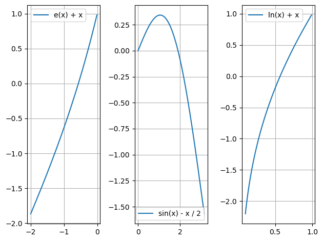
On reprend les fonctions:

• \(f(x) = \exp(x) + x\)

• \(g(x) = \sin (x) - x / 2\) avec \(x > 0\) à \(10^{-12}\) près.

• \(h(x) = \ln (x) + x\) à \(10^{-12}\) près.

from scipy.optimize import bisect

def f(x):
    return np.exp(x) + x


def g(x):
    return np.sin(x) - x/2


def h(x):
    return np.log(x) + x


"""Etude graphique"""
xf = np.arange(-2, 0, 1e-2)
xg = np.arange(0, np.pi, 1e-2)
xh = np.arange(0.1, 1, 1e-2)
fig, ax = plt.subplots(1, 3)
ax[0].plot(xf, f(xf), label="e(x) + x")
ax[1].plot(xg, g(xg), label="sin(x) - x / 2")
ax[2].plot(xh, h(xh), label="ln(x) + x")

ax[0].legend()
ax[1].legend()
ax[2].legend()

ax[0].grid()
ax[1].grid()
ax[2].grid()

fig.tight_layout()
plt.show()

xf1 = dicho_while(f, -2, 0, 1e-12)
xf2 = dicho_recursif(f, -2, 0, 1e-12)
xf3 = bisect(f, -2, 0)

xg1 = dicho_while(g, 0.1, np.pi, 1e-12)
xg2 = dicho_recursif(g, 0.1, np.pi, 1e-12)
xg3 = bisect(g, 0.1, np.pi)

xh1 = dicho_while(h, 0.1, 1, 1e-12)
xh2 = dicho_recursif(h, 0.1, 1, 1e-12)
xh3 = bisect(h, 0.1, 1)

print("Racine de f : {}".format([xf1, xf2, xf3]))
print("Racine de g : {}".format([xg1, xg2, xg3]))
print("Racine de h : {}".format([xh1, xh2, xh3]))

Nombre d iterations : 41
Nombre d iterations : 42
Nombre d iterations : 40
Racine de f : [-0.5671432904096037, -0.5671432904096037, -0.5671432904109679]
Racine de g : [1.8954942670342385, 1.8954942670342385, 1.8954942670332011]
Racine de h : [0.5671432904096492, 0.5671432904096492, 0.5671432904100584]

_Note : on remarquera que les valeurs sont à peu près égales à \(10^{-12}\) près mais pas rigoureusement car le test d’arrêt dans bisect est un peu plus complexe que la simple largeur de l’intervale.