La page ci-présente existe en version notebook téléchargeable grâce au bouton (choisir le format .ipynb). On rappelle qu’il faut ensuite l’enregistrer dans un répertoire adéquat sur votre ordinateur (capa_num par exemple dans votre répertoire personnel) puis lancer Jupyter Notebook depuis Anaconda pour accéder au notebook, le modifier et exécutez les cellules de code adéquates.

3.3. Exemple d’implémentation basique

3.3.1. Implémentation

from numpy import *
from matplotlib.pyplot import *
from scipy.integrate import odeint

def euler(f:callable, y0:float, t0: float, tf: float, pas:float) -> (ndarray, ndarray):
    tk = [t0]
    yk = [y0]
    while tk[-1] < tf:
        yk.append(yk[-1] + f(tk[-1], yk[-1]) * pas)
        tk.append(tk[-1] + pas)
    return array(tk), array(yk)

3.3.2. Utilisation

def f(t, y):
    return - sin(t) * y + 2

y0 = 0
t0 = 0
tf= 10
pas = 0.1
tk , yk = euler(f, y0, t0, tf, pas)
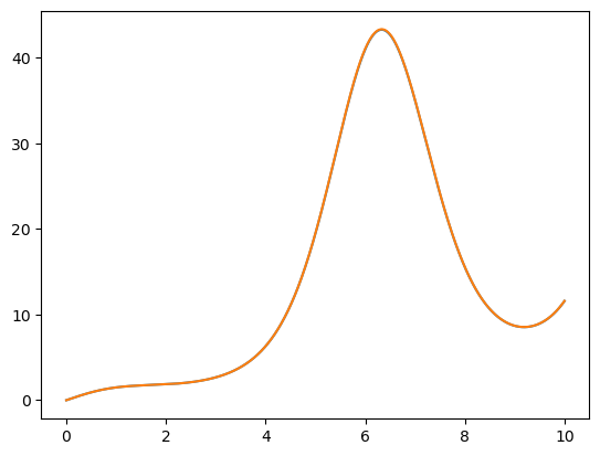
plot(tk, yk)

yk2 = odeint(f, [y0], tk, tfirst=True)
plot(tk, yk2)

[<matplotlib.lines.Line2D at 0x1f351466df0>]

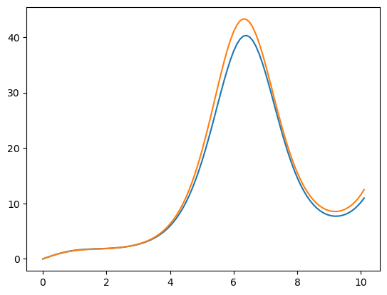
On remarquera une légère différence car odeint utilise une méthode plus précise. Cette différence s’estompe avec un pas pus faible (cf. suite)

pas = 0.001
tk , yk = euler(f, y0, t0, tf, pas)
plot(tk, yk)

# Résolution avec odeint
yk2 = odeint(f, [y0], tk, tfirst=True)
plot(tk, yk2)

[<matplotlib.lines.Line2D at 0x1f3515750a0>]

t, y = linspace(min(tk),max(tk),20), linspace(min(yk),max(yk),20)
tgrid, ygrid = meshgrid(t, y)
quiver(tgrid, ygrid, ones((len(t), len(y))), f(tgrid,  ygrid), angles='xy')
plot(tk, yk)

[<matplotlib.lines.Line2D at 0x1f3515340a0>]

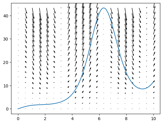
Les “flèches” représentent la valeur de \(f\), dont bien la pente puisqu’il s’agit de la dérivée.

# avec solve_ivp
from scipy.integrate import solve_ivp
pas = 0.001
tk , yk = euler(f, y0, t0, tf, pas)
plot(tk, yk)

tks = arange(t0, tf, pas)
# Résolution avec odeint
yk2 = solve_ivp(f, (t0, tf), [y0], t_eval=tks)
plot(tks, yk2['y'][0])

[<matplotlib.lines.Line2D at 0x1f352e43f70>]